
ALMA Imaging Tutorial: Z-CMa
Z Canis Major (or Z CMa) is young binary system in the constellation Canis Major. The binary consists of two pre-main sequence stars, one of the classification Herbig Be star and the second a FU Orionis object.
A Herbig Ae/Be stars are young enough to still be embedded in their contracting natal dust and gas envelopes and to not yet be burning hydrogen. FU Orionis objects show highly variation in magnitude and spectral type potentially linked to episodic accretion from their accretion disks onto the star.
Both objects in Z CMa drive outflowing jets which can be well traced by molecular line emission observable by ALMA. In this tutorial we will use ALMA observations of Z CMa to image the gas/dust continuum emission and the 13CS and CO spectral line emission. The latter giving some insight into the outflowing material structure.
The ALMA observations we are using were conducted under project code 2018.1.01131.S on 14-March-2019 in ALMA Band 6 (using frequencies between ~218.2-232.5GHz). The full project consists of both 12M and 7M array data, but for this tutorial we will focus only on the 12M data.
Getting started:
As discussed earlier in this workshop we will be using CASA to image these data. You should have CASA installed and checked that it starts successfully before the start of this session. You will also need the imaging script 'scriptForImagingZCMa.py' and a CASA measurement sets (MSs) containing the data.
Whilst these data are fairly typical in terms of file size for an ALMA observation, we know people have differing computing resources. As such we provide two options of starting data which can be used as follows.
1) uid___A002_Xd98580_X354.ms.calibrated (untarred file size 31GB). This is the end product of running scriptForPI.py as discussed earlier in this workshop. Here you can work from Step 0 to the end of the tutorial. The final data products will have a size of approximately 70GB, so make sure you have enough room for this on your computer.
2) Z_CMa_TM2.split.cal (untarred size 5.8GB). This is the science target only data and is created in the first half of Step 1. If you start with this MS you can follow the hands-on part of this tutorial from the ∀ symbol. If you select this product please be sure to still read Step 0 and the start of Step 1. The final data products starting with these data will have a size of YGB.
Once you have downloaded and untarred you data, please start CASA.
About this tutorial:
This tutorial follows the steps in the scriptForImagingZCMa.py we have provided. There is a 'switch' for each step on lines 56 to 61 of the script which need to be set equal to True if you wish to run that step and False if not. Typically, you should run one step at a time and in the order they are listed.
Also, to allow you to get some hands-on experience a number of parameters used throughout this script are left blank and need to be set by you. These all appear under the heading `Initial Parameters' on lines 35 to 50 of the code. Don't worry we will guide you has to how to calculate or find the required values.
STEP 0: Obtaining and inspecting the data
If you have successfully run the scriptForPI.py on the downloaded data you will have in the /calibrated/ directory a measurement set (MS) named 'uid___A002_Xd98580_X354.ms.calibrated'. If scriptForPI.py failed to run (or you didn't have enough disk space) the full MS can be found here (untarred file size 31GB). If you lack disk space for this MS please read the remainder of this step and Step 1, you can proceed with the hands-on elements of this tutorial part way through Step 1 at the ∀ symbol.
Our first step is to inspect what this MS contains. The CASA task listobs can be run to do this. You can run this directly in the CASA terminal as follows:
listobs('uid___A002_Xd98580_X354.ms.calibrated')
This will print a lot of useful information about the observation into the CASA logger. Another way of running listobs is used in Step 0 of the tutorial script. Before running this step we need to set the following values in the 'Initial Parameters' section of the script.
myMS = 'uid___A002_Xd98580_X354.ms.calibrated'
target = 'Z_CMa'
These values are used throughout the script. Next we need to set the parameter step0 = True in the 'Logic switches' section of the code. With these set, let's have a look at the slightly different listobs command used in Step 0.
listobs(myMs,listfile=myMS+'.listobs')
Here we use the myMS variable we set above, rather than writing out its full name each time, and we set the listobs parameter listfile to be the MS name plus the extension .listobs. This will produce a text file named 'uid___A002_Xd98580_X354.ms.calibrated.listobs' which contains the same information as was printed to the terminal in the previous listobs command.
To execute this step of the script type:
execfile('scriptForImagingZCMa.py')
into CASA. Once it has finished you can open the file 'uid___A002_Xd98580_X354.ms.calibrated.listobs' in your favourite text editor. We'll go through the file now...
STEP 1: Split out science target and science SPWs
Inspecting the .listobs made in step 0 you will see it contains a lot of data we won't need when imaging the source. For example, myMS contains scans on the calibrators used during observation and spectral windows (SPWs) which are used only for calibration steps. To give us a smaller MS to work with we will `split' out from myMS just the data relating to the target source and the science SPWs.
We can find the `science only' spectral windows 'by-hand' using the information in the .listobs file created in Step 0. Or we can use a handy Python function named getTargetSciSPW which is included in the tutorial script, scriptForImagingZCMa.py. The first part of Step 1 finds the science spectral windows with this function and then splits out just those SPWs and data related to the target (the name of which we set in the previous step).
scispws = getTargetSciSPW(myMS)
print '>> scispws: '+scispws

split(vis=myMS,
 intent = 'OBSERVE_TARGET#ON_SOURCE',
 datacolumn='corrected',
 field=target,
 spw = scispws,
 outputvis=target+'_TM2.split.cal')
Using the above commands we generate a new MS called 'Z_CMa_TM2.split.cal'.
We can now generate a new .listobs file for this MS with the command:
listobs(target+'_TM2.split.cal',listfile=target+'_TM2.split.cal.listobs')
You will notice when inspecting the new .listobs file that the SPWs numbers from scispw have now been shifted down to 0-10.
To run this step from the script set step1 = True and all other steps to False and type:
execfile('scriptForImagingZCMa.py')
∀ If you did not have enough disk space for the whole MS in Step 0 a copy of 'Z_CMa_TM2.split.cal' can be downloaded here (file size 5.8GB untarred), you can proceed with the hands-on tutorial from here.
For those starting here, make sure you have set the myMS and target variables in your script as described in Step 0 and then you can enter this command into your CASA terminal to generate your copy of the new .listobs file.
listobs('Z_CMa_TM2.split.cal',listfile='Z_CMa_TM2.split.cal.listobs')
From this point on, everyone can follow exactly the same steps.
STEP 2: Inspect science SPWs for spectral line emission
To perform accurate science with any detected spectral lines we need to work with continuum subtracted data; conversely to do reliable science with the continuum emission we need to use only spectral line free channels. As such, we next inspect each SPW to see if there is a spectral line detection and to look for any obvious continuum emission within the data.
To inspect the data we need to use the CASA task plotms. This is CASA's general purpose plotter for the visibility data, to open plotms you just need to type plotms in the CASA terminal. Now we need to tell plotms what to plot.
First, on the "Data" tab (the first which opens when you start plotms) click the Browse button and select your newly created .split.cal MS. In the "Averaging" panel below select time and enter in the text box a LARGE value (something greater than the total on source time for the observations, e.g 1e8 [which is about 3 years 2months in seconds]). Also select 'All Baselines'.
These two values will average your visibilities in both time and across all array baselines giving plotms far fewer points to plot. (NOTE: Always be careful with plotms, it will try and plot whatever you tell it, but without averaging the number of data points can be in the several millions to billions!).
Next, we select the axes we want, in the 'Axes' tab down the left hand side of the GUI. Set x-axis as Channel and y-axis as Amp, meaning we will plot the visibility amplitudes as a function of channel.
Finally, select the 'Page' tab down the left hand side and set the 'Axis' value in the 'Iteration' panel to 'Spw', this will tell plotms to plot one SPW at a time, for easier inspection. Finally click on the 'Plot' button at the bottom.
Let plotms do its thing for a minute or two (we still have a lot of data points to plot (approx 12e6)). When it loads you can page through each SPW using the green arrows along the bottom of plotms.
Whilst plotms is loading, Figure 1 gives an example of the 'line free channels' which we wish to make note of for both imaging the continuum (Step 3) and continuum subtraction and line imagine (Step 4).

Fig1: Synthetic spectrum plotted as Channel vs Flux Density. The line free channel ranges are noted by the black lines and channel values.
For this simple case the line free channel are 0 to 90, 150 to 280, 317 to 370 and 430 to 510. In CASA syntax this would be written as SPW No.:0~90;150~280;317~370;430~510 (where 'SPW No.' would be replaced by the SPW number and remember these are not the values to use with our data).
Once plotms has loaded all the plots for our data set, you should see something like these example plots (one for each SPW if you use the green arrows to move back and forth between them):
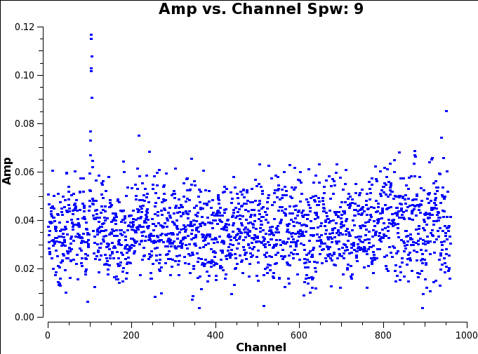
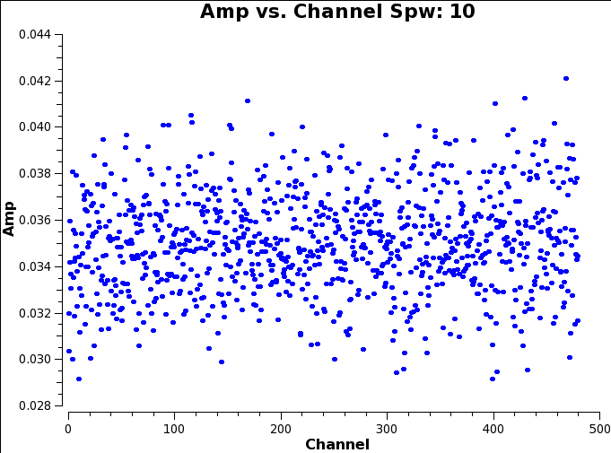
It seems that there is a good level of continuum in this source (all SPWs have visibility amplitudes offset from 0. And there are two clear line detections in SPWs 8 and 9.
SPW 8 is CO(2-1) at 230.538GHz (shifted to the source rest velocity of -27km/s)
SPW 9 is 13CS at ~231.2206GHz
In terms of channels the CO line appears in SPW 8 from channel shortly after channel 0 to around 250. As such, and to add a little buffer we can say the line free channels in SPW are are from 300 to 959 (there are 960 channels in this SPW and CASA starts counting at 0). In CASA syntax this channel range can be written as 8:300~959.
Similarly, for the much narrower line in SPW 9 we see the emission between channels 90 and 110. This gives us line free channels (again with a bit of a buffer) of 9:0~85;115~959. Notice here we have defined two line free channel ranges either side of the line and separated them by a semi-colon.
All the other SPWs are empty of spectral line emission, and so we can use all available channels when continuum imaging. Given this we can write a single string which defines all the line free channels across all the SPWs in the data set. In CASA syntax you separate SPWs in such a string with a comma. If you want to include all channels from a given SPW you just need to provide its SPW number. So for Z_CMa we can define a variable called contSPW which lists all the channels, in all SPWs, which are spectral line free as:
contSPW = '0,1,2,3,4,5,6,7,8:300~959,9:0~85;115~959,10'
Remember to fill this in the `initial parameters' section of your copy of ScriptForImagingZCMa.py.
STEP 3: Image continuum
The first step in any imaging is to calculate the required imaging parameters cell, imsize and threshold. The first two define the size of the pixels in the image we are going to make and the total size in pixels of that image, respectively. The third helps to constrain the tclean algorithm so that we don't over clean our data. To calculate these values we need to know the following properties of our data: The field of view (FoV), the expected resolution, the number of antennas used during observation, the total time on source, the frequency bandwidth and the system temperature during our observations.
Field of View and Resolution
The observed FoV is approximately the same as the primary beam size of a single antenna in our array at our observing frequency. For this we need to know the Diameter of our ALMA antennas. For these data, we have 12m ALMA dishes and we can use the average frequency value of the 10 SPWs we are going to image simultaneously (224.35GHz or converted to wavelength 1.336mm). Thus our FoV ~ wavelength/12.0 ~ 23.0arcsec.
Similarly we need the expected resolution, for which we need to know the maximum baseline of our observation. To do this we can use a task from the Analysis Utilities package called getBaselineLengths() as follows:
blines = aU.getBaselineLengths(target+'_TM2.split.cal')
This function returns the maximum baseline length, b_max, of 360.56m. Our resolution (res) is then , res ~ wavelength/b_max ~ 0.76arcsec. To ensure we sample our data well over the beam we want to have greater than 3 pixels across the beam. We set the pixel size using the cell parameter in tclean. Typically ALMA tries to use between 5 and 6 pixels across a beam. Set the cell value in your copy of the ScriptForImagingZCMa.py script.
To get our imsize in pixels we divide or FoV by cell size = 23.0/cell, we can then set imsize to approx twice this. Note: tclean in CASA has some 'preferred' image sizes, which make tclean work more quickly. The tutor will now show these on the screen, please select the closest value to your calculated imsize.
We can now fill in the myCell, myImsize values in the `initial parameters' section of the script. To be used by the tclean command at step 3.
Estimating a cleaning threshold
Interferometric imaging works best when the tclean task is given some sensible constraints. Primarily these take the form of tclean mask (as discussed in the imaging tutorial<link>) and a threshold on the amount of cleaning which is undertaken. We will set the former interactively during the tclean, but the latter can be set beforehand.
Two parameters can limit the amount of cleaning which gets done, they are niter and threshold. niter sets the number of iterations of clean which can be done, so making this a small number means only a small amount of cleaning is done. Whilst this method has its uses, it is hard to know a priori how many clean cycles are enough. The second limiter on the amount of cleaning undertaken is the parameter threshold. This sets an absolute noise value which when reached within you clean mask the algorithm will stop. Combining threshold with a reasonable niter value (several thousand) means CLEAN will stop either when the noise limit is reached or some (but not too many) iterations of clean have occurred.
So, how do we calculate a sensible noise threshold? A reasonable first estimate is a few times the theoretical RMS noise of your observation. We can calculate this from the available data in our listobs file (plus one other value). From the listobs we need the number of antennas used (Nants), the time on source (Δt), the total bandwidth (Δν).
Nants can be read straight from the listobs file itself. The 'timerange' of the on source scan is also given in listobs, so we can trivially convert that to a time on source (in seconds). Finally, to calculate our total bandwidth we need to take the number of channels we are using in each SPW (after excluding channels with lines emission STEP 2) and multiply this by the channel width (ChanWid in listobs) in that SPW. The total bandwidth is then the sum of these values for each SPW. We need this total bandwidth in unit Hz.
The final value required to calculate a theoretical RMS is an approximate value of the system temperature (Tsys). This is not as easy to find, and the easiest approach is to look in the weblog (discussed in X tutorial) which normally be downloaded with your data when you take it from the ALMA Archive. In the case of these data we want to look at the plots in Step 6 of the weblog and estimate the average Tsys across all antenna and SPW.
Given all of these values the theoretical RMS noise can be calculated as:
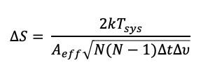
Equation 1: Theoretical sensitivity of an interferometric image.
where, in addition to the variable discussed above, k is the Boltzmann constant and Aeff the collecting area of a single dish in your array (times ~0.7 to account for various efficiency parameters). N = Nants.
We can then set the threshold to 3 or 5 (or more) times this value as the parameter myThreshold in scriptForImagingZCMa.py.
With myCell, myImsize and myThreshold set we can start running tclean on our data. To do this set step3 = True (all others to False) in the script and type the following command into your CASA terminal:
execfile('scriptForImagingZCMa.py')
tclean will then start running interactively and you can proceed through cleaning as described in the Imaging tutorial. Whilst this step is running please take a look at the tclean command used to generate the continuum image, the tutor will discuss the choice of parameters which have been set for you.
The UK ARC Node tutors will be on hand (Zoom or Slack) to answer any questions you have during the cleaning stage.
STEP 4: Spectral line imaging
Imaging the spectral lines we found in Step 2 accurately first requires us to remove any continuum emission from our data. This is done using the CASA task uvcontsub, the specific command is given in Step 4 of ScriptForImagingZCMa.py and looks like this:
uvcontsub(vis=target+'_TM2.split.cal',
               fitspw = contSPW)
This task will fit a first order polynomial to visibility data in each SPW using only the channels we define in our contSPW variable. It then subtracts from the visibilities the generated fitted to remove the continuum emission and creates a new MS called target+'_TM2.split.cal.contsub'. This is the MS which we will use for spectral line imaging.
We will then proceed to image both the CO and the 13CS data cubes. We refer to the products as cubes as they have three dimensions, Right Ascension, Declination and Velocity/Frequency.
Before running this step there are some parameters you need to fill in within the script. First we need to redefine the threshold for cleaning, one for each spectral line giving us myThreshCO and myThreshCS. Now you will note from Equation 1. that the only thing which changes between our previous calculation of a noise threshold and these is parameters is the bandwidth. For spectral cubes we want Δν to be the width of a single channel. Given this we can simply scale our previous threshold by the ratio of the Δν for continuum and Δν for spectral cubes. The channel width for the CO and 13CS SPWs can be found in the .listobs file.
The last thing to set are the start channel and number of channels (parameters start and nchan in tclean), we define these in the initial parameters section of the script as nChanCO, startCO, nChanCS and startCS for CO and CS respectively. the value startCO tells tclean which channel to start making the cube from and nChanCO how many channels after the start channel to image (and the same for the 13CS values). We can return to plotms as we did in step 2 to confirm the channel ranges for the two lines.
With the thresholds, starts and nchans set for both species you can then run Step 4 by setting step4 = True (all others to False) and typing the execfile command in the CASA terminal. This time we are using CASA's automasking capabilities to draw the clean boxes for us. The tutor will run through how this works and the differences in the tclean command for spectral cube imaging as your cubes are being made.
STEP 5: Advanced imaging steps
The final step in this tutorial is to create some "Advanced imaging" products. Specifically, zeroth, first and second order moment maps. The definitions for each of these moments (and several more) can be found here, but simply they translate to the integrated intensity of your line (zeroth), velocity field/gradient (first) and velocity dispersion (second).
In this step we want to make two sets of the moment maps, one at the red shifted and one at the blue shifted side of Z-CMa in CO. To do this we can open up the CO cube we made in the previous step and inspect both the cube and the spectrum of the line. You can use either CASA's viewer or CARTA to do this.
The last two parameters you need to set for this tutorial are those named myChansRed and myChansBlue. Using the spectrum of CO you can define channel numbers to make the image moments over. Note: Here we are talking about channels in the cube, not the channels from the CO SPW. The we use the immoments task in Step 5 to create these moment maps. The chans parameter of immoments uses the same syntax as the spw parameter we have seen before to define channel ranges. So to take the moment(s) for channel X to Y then we need to write 'X~Y'.
When you have set myChansRed and myChansBlue you can run Step 4 by setting step5 = True (all others to False) and typing the execfile command in the CASA terminal.